Terrain Visualization Modes

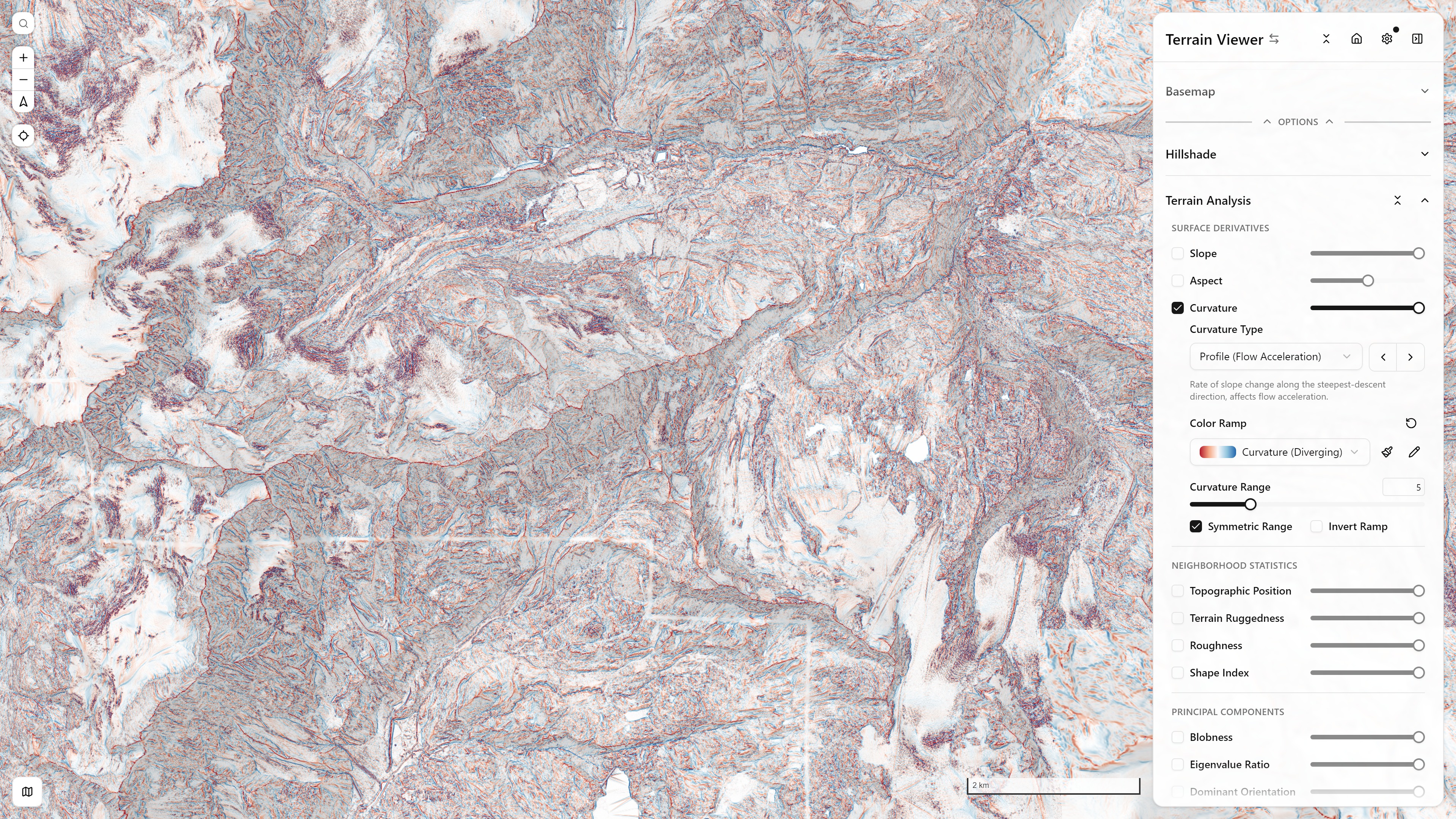
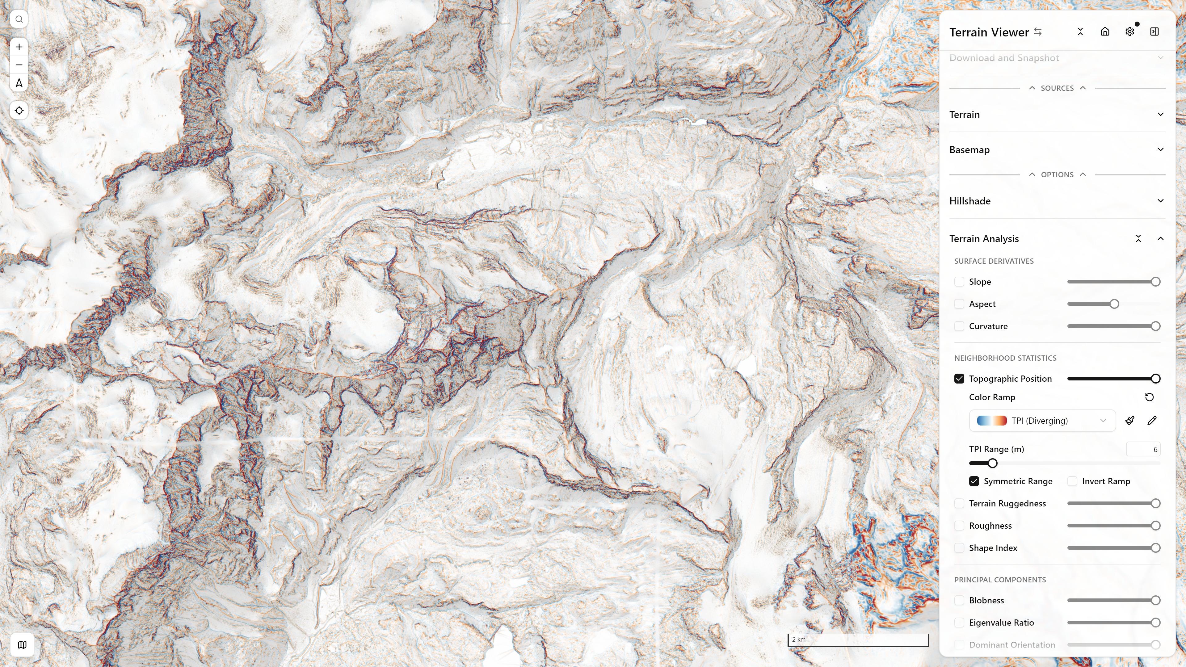
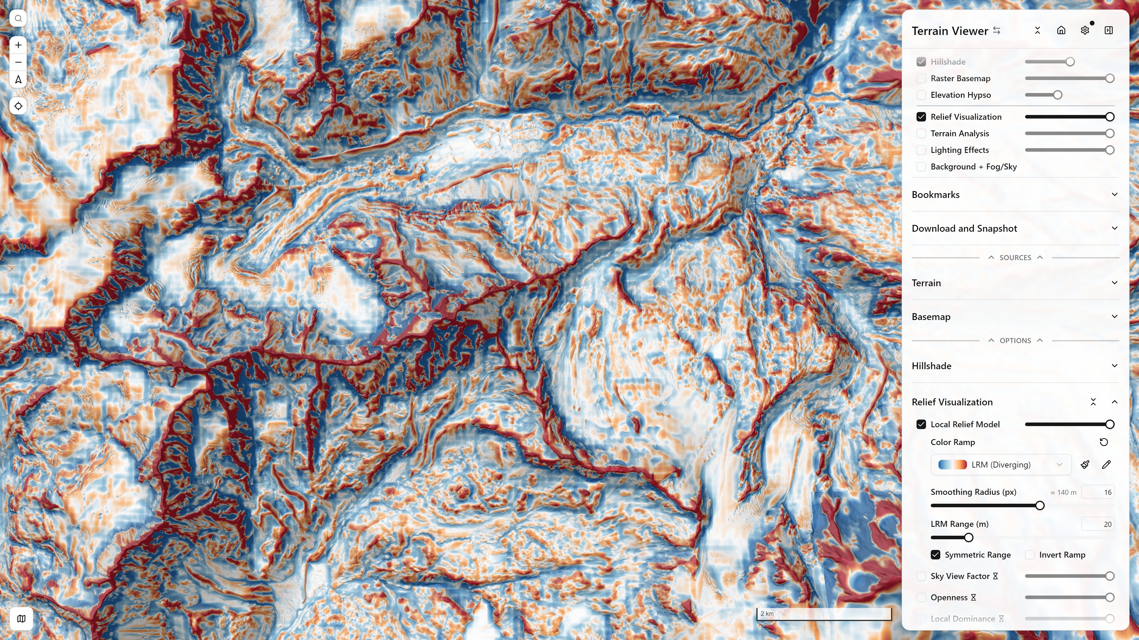
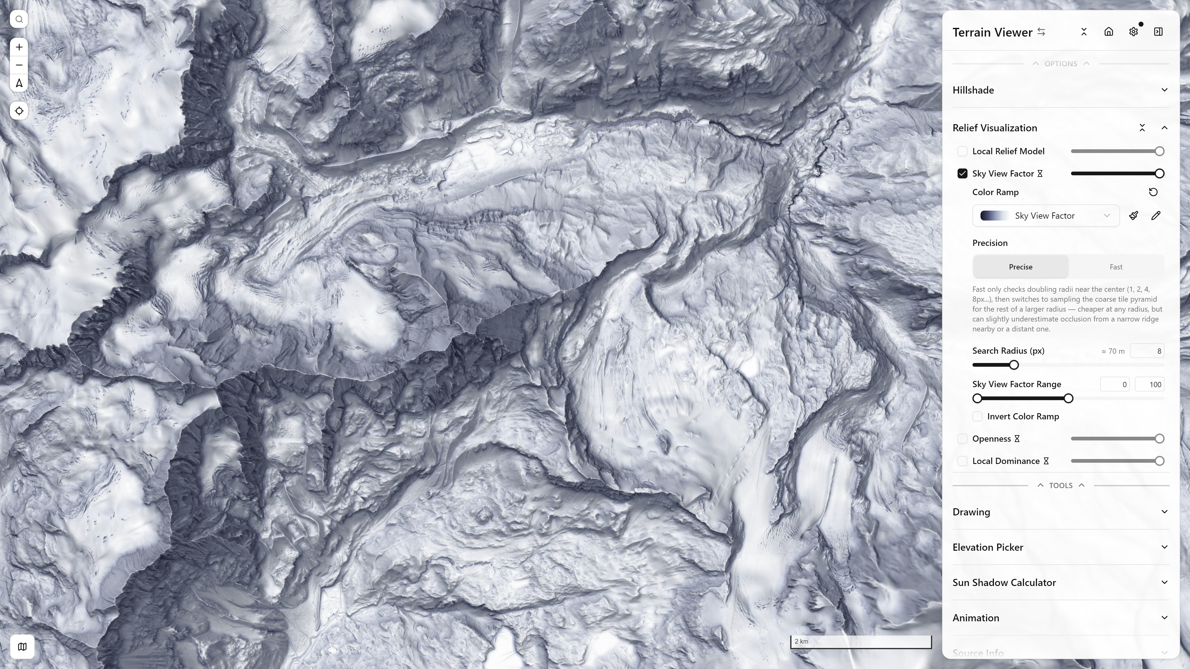
Most of these are inspired by gdaldem and the RVT (Relief Visualization Toolbox) QGIS plugin. "Neighborhood" usually means a 3×3 kernel centered on the pixel. Every mode stacks over the terrain/basemap and over each other — for the terrain-analysis, relief, and light rows below, all share the same viewport (Matterhorn massif, Switzerland/Italy) and a 20% Hillshade backdrop (except where Hillshade would be redundant), so the underlying terrain is directly comparable mode to mode:

Data layers pickerCopy Anchor Link

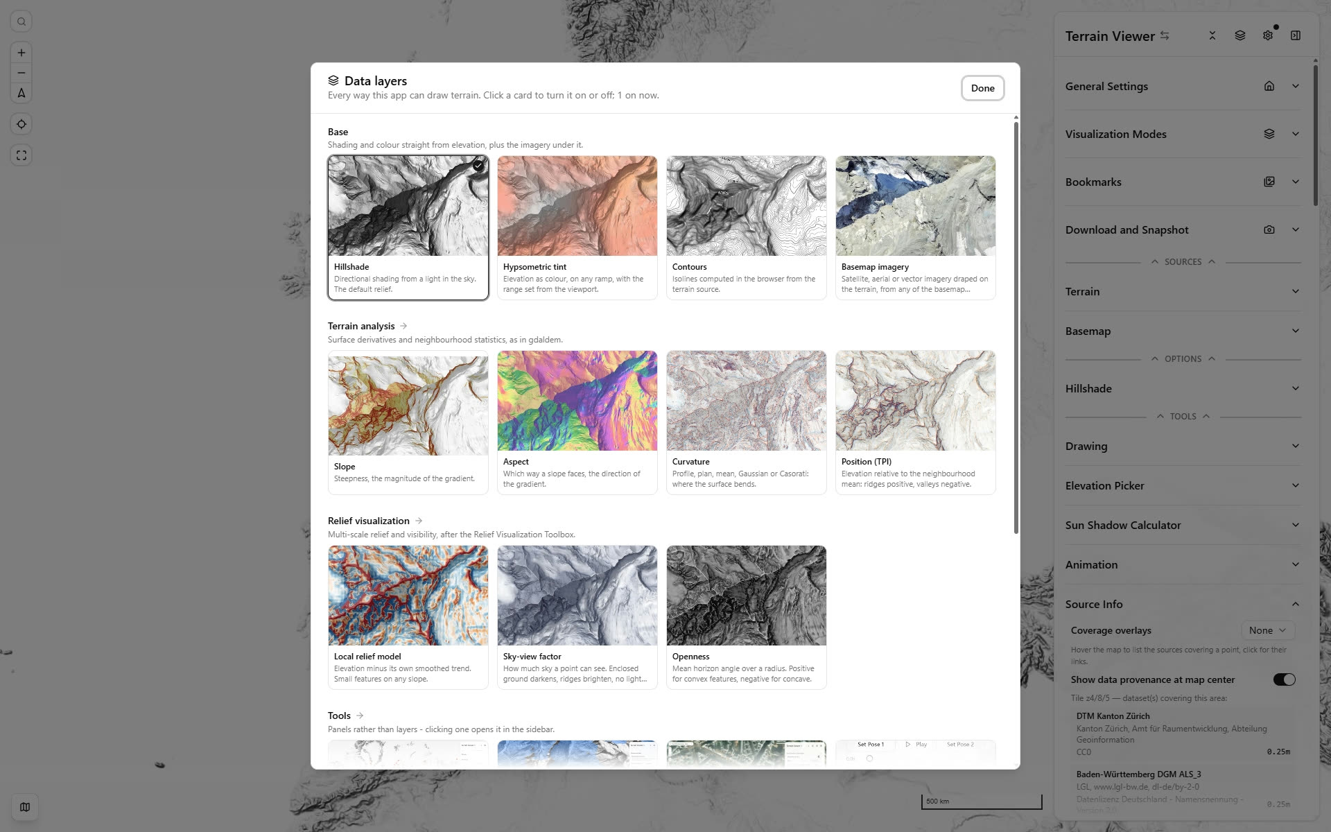
The Data layers picker - every visualization mode as a card of the same Matterhorn view, plus a Tools row

Every mode on this page is also a card in the Data layers picker — the Layers button in the panel’s title bar, or next to the Visualization Modes pin. Each card is a thumbnail of the same Matterhorn view with only the rendering changed, so the modes can be compared before any is switched on; clicking a card toggles it (and switches on the section it belongs to). Group titles — Terrain analysis, Relief visualization, Light, Tools — open that section in the sidebar, and the Tools row does the same for Draw, Elevation picker, Sun shadow and Animation. Modes without a screenshot yet (Ruggedness, Roughness, Blobness, Local dominance) are only in the sidebar.

The thumbnails are 640 px crops of the docs’ own captures (docs/scripts/build-screenshot-thumbs.mjs), and the captures themselves are reproducible from docs/scripts/capture-viz-mode-cards.mjs, which uses the parameters linked under every screenshot here.

Combined ModeCopy Anchor Link

Every mode above is independent — any number can be on at once, each with its own opacity slider right there in the Visualization Modes checklist, so a Hillshade backdrop, a color ramp, and a derivative can all be dialed in together rather than picked one at a time.

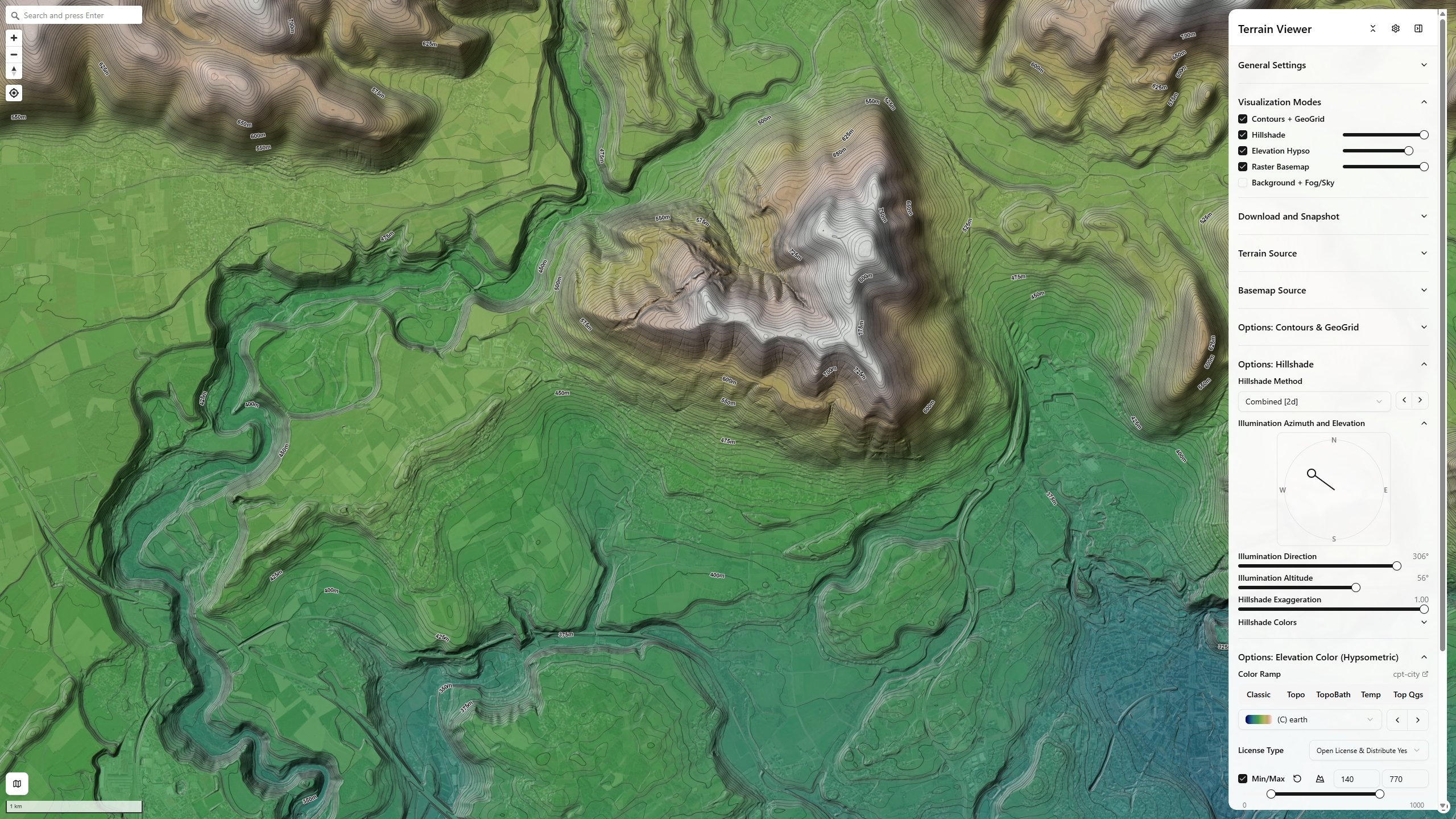
Combined mode — Contours + Hillshade + Elevation Hypso + Raster Basemap stacked together, Karakoram/Himalaya

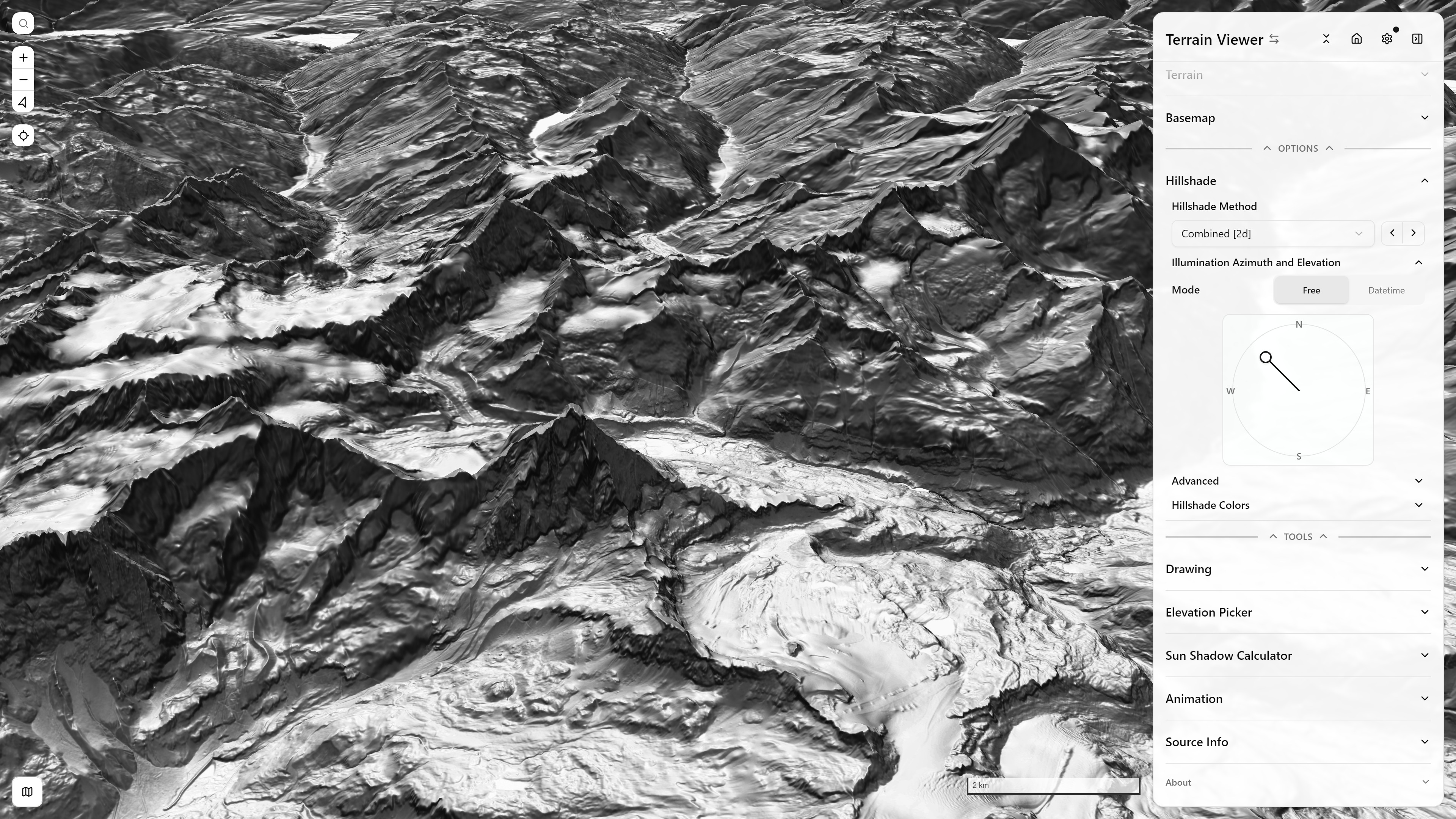
HillshadeCopy Anchor Link

Native MapLibre hillshade with multiple illumination methods (Standard, Combined, Igor, Basic, Multidirectional, a colored/aspect-tinted variant, and Duotone NW/NE: a grey north-west light plus a north-east light whose lit side is blue and shaded side orange, after Čučković's two-light LiDAR hillshade) — see MapLibre PR #5768.

Hillshade — dragging the XYPad to set light azimuth/elevation

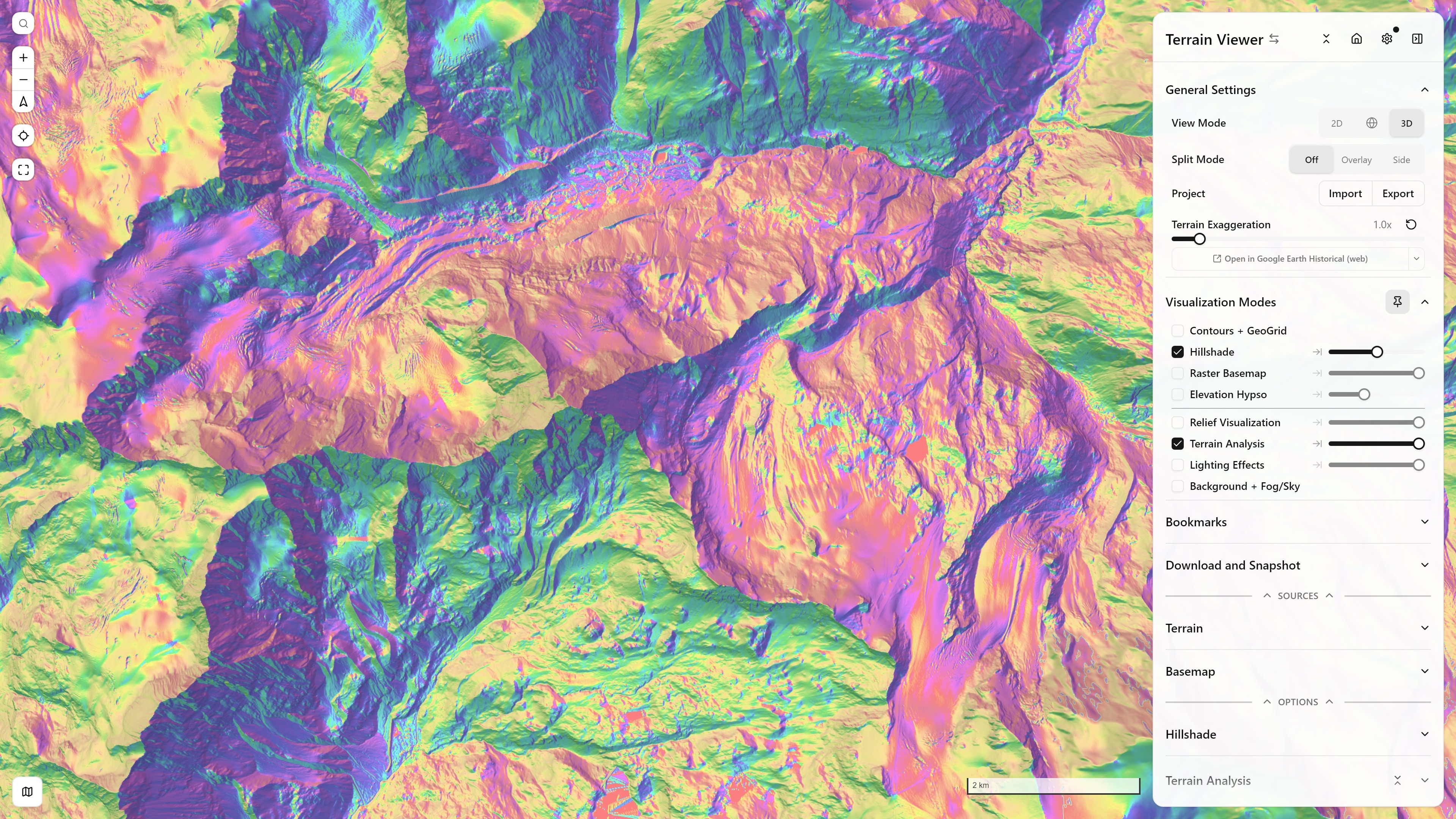
Terrain Analysis — Aspect over Hillshade, plan view, Matterhorn massif — open this view

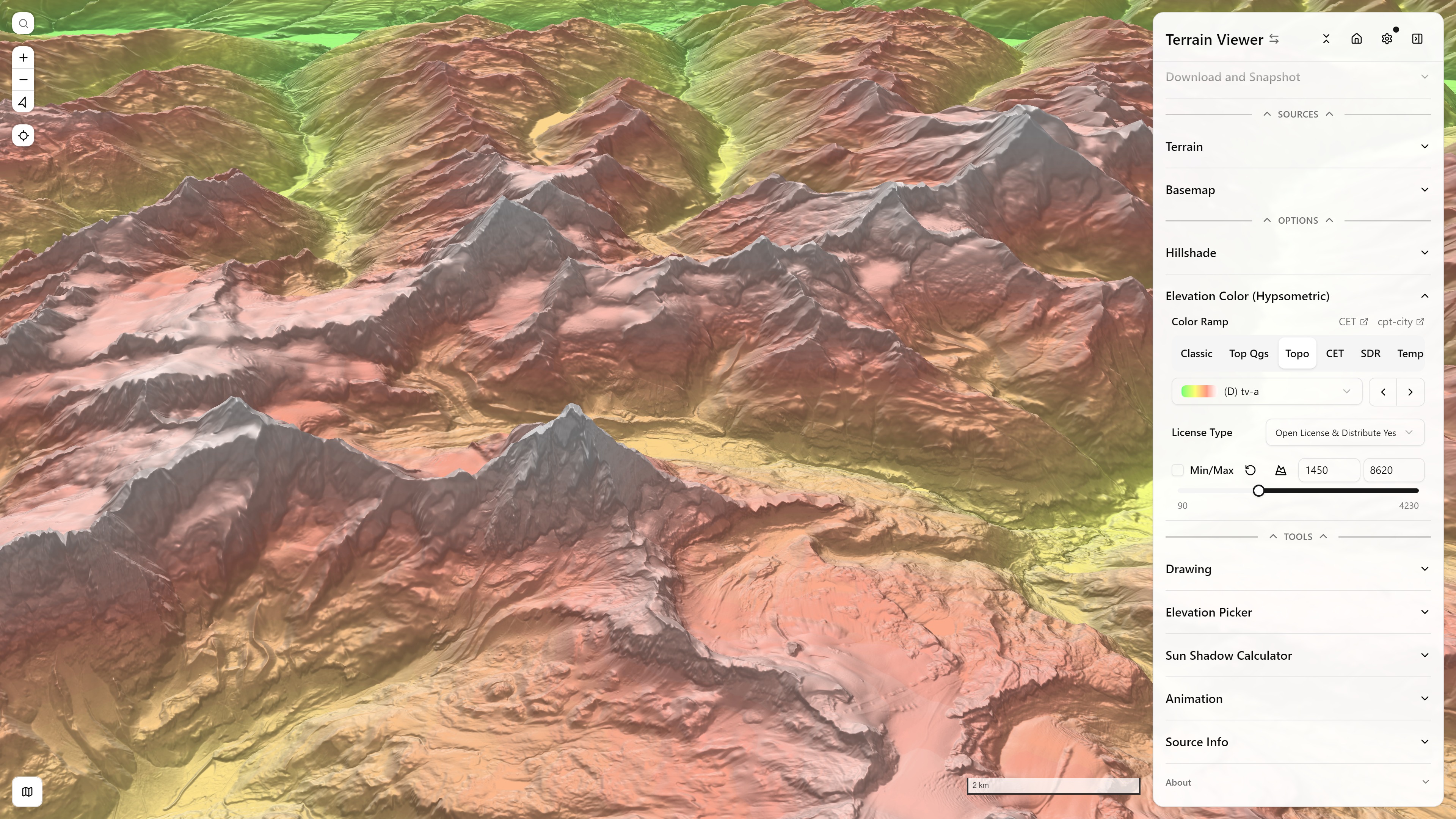
Elevation Hypso (Hypsometric Tint)Copy Anchor Link

Color-encoded elevation with a choice of color ramps (including CPT City ramps, and in the Classic tab Relief Green-Red, the green-to-red palette of archaeological LiDAR figures: pale cyan for water and the lowest ground, greens, yellow and orange up to a dark red top) — see MapLibre PR #5913.

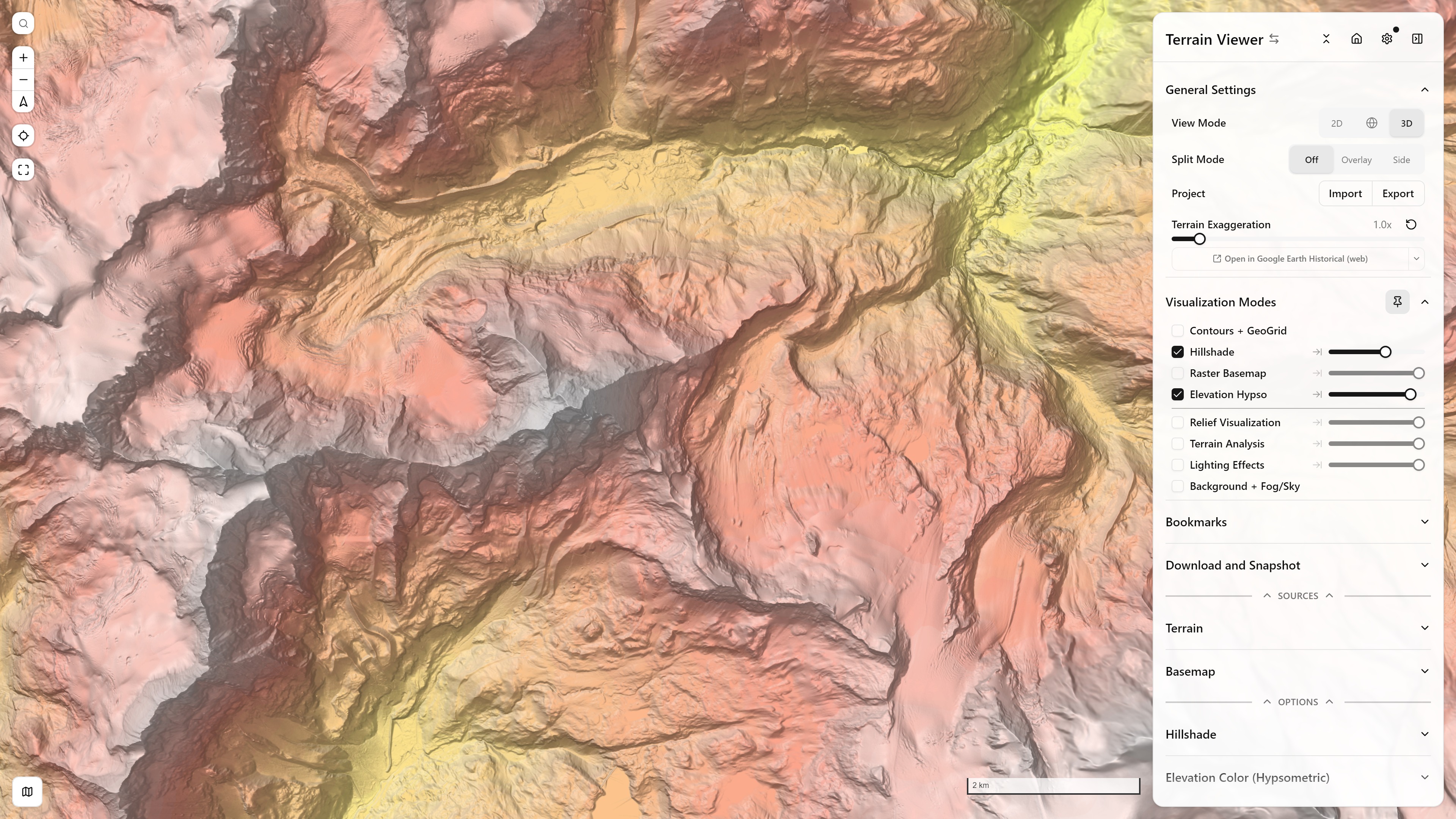
Elevation Hypso + Hillshade, with the Elevation Color controls panel open — Matterhorn massif — open in app ↗

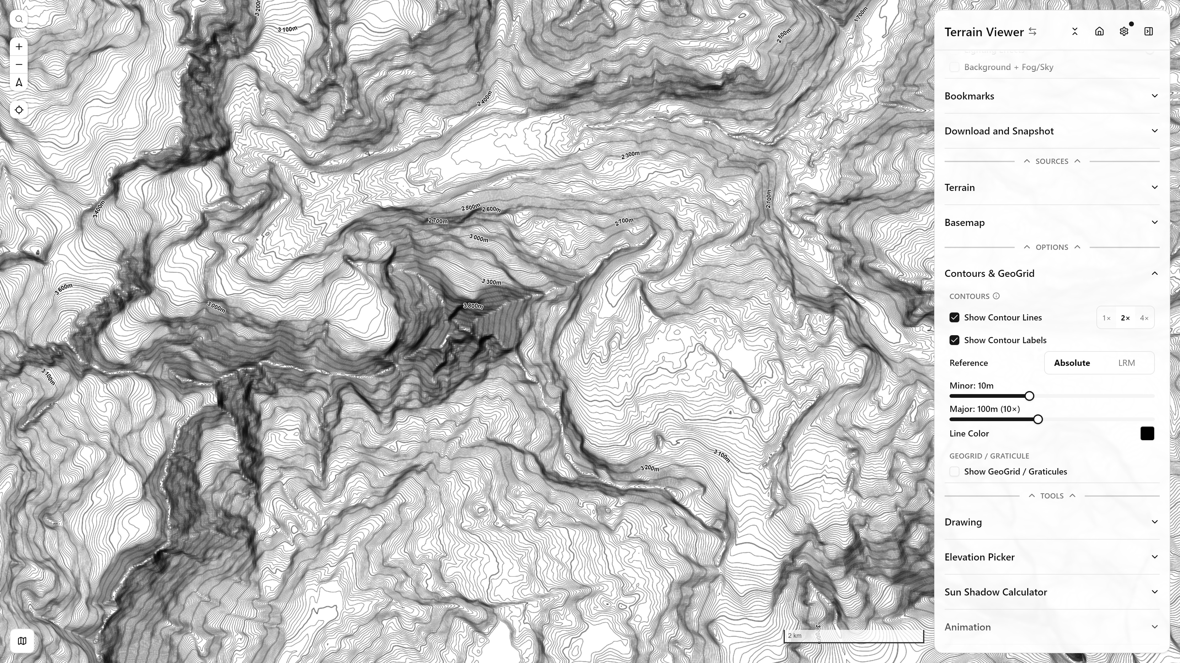
Contours + Geo GridCopy Anchor Link

Contour lines trace one of two references. Absolute is real elevation, with a minor and a major interval. LRM traces the Local Relief Model instead, so the lines follow local bumps and hollows rather than altitude.

Configurable-interval contour lines via onthegomap/maplibre-contour, plus a lat/lng graticule overlay.

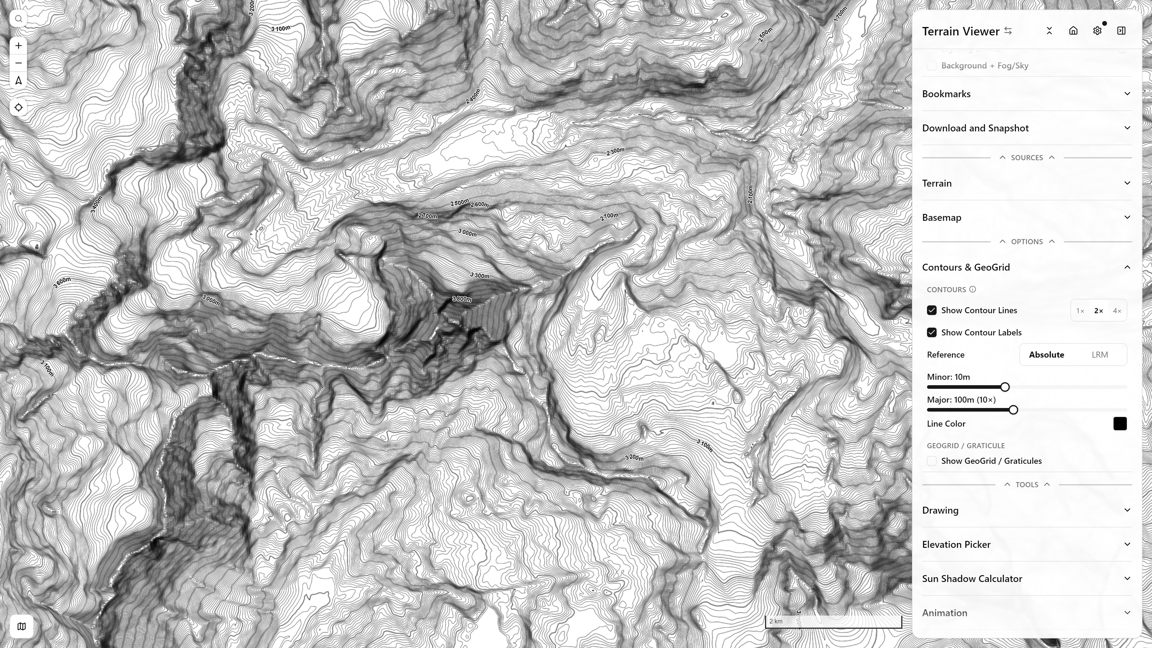
Contours + GeoGrid alone (no Hillshade), top-down, with the Contours & GeoGrid controls panel open — Matterhorn massif — open in app ↗

Iso-lineCopy Anchor Link

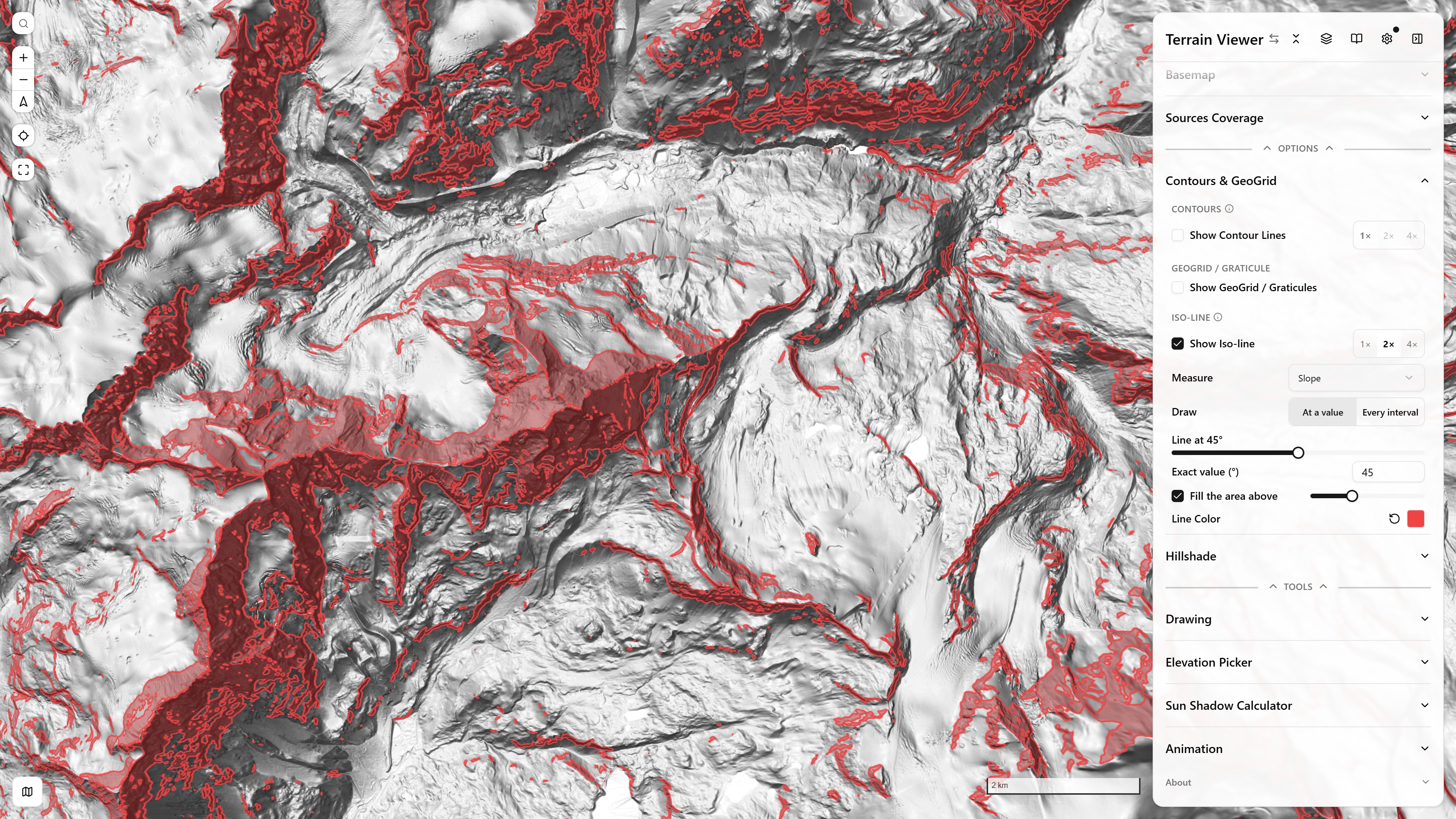
Iso-line, Slope at 45° with Fill the area above, over Hillshade, with the Contours & GeoGrid panel open, Matterhorn massif · open in app ↗

Iso-line is the third group of Contours & GeoGrid, under the geogrid (Show Iso-line): a vector line drawn from any measure, independent of the contour lines. The measure is the elevation, any terrain-analysis mode (slope, aspect, TRI, TPI, roughness, curvature, shape index, blobness, eigen ratio, orientation), the local relief model, or a lighting mode's brightness (Phong with its rim, Matcap, the hard shadow), each with that mode's own settings (the curvature kernel, the LRM radius, the light, the Phong strengths and Fresnel rim). The horizon modes (sky-view factor, openness, local dominance) are left out: minutes per view at the zooms a line needs. At a value draws one line where the measure crosses the value you set (an iso-slope at 30° for avalanche terrain or 80° for cliffs, a lake or flood level, canopy on an nDSM at 1.5 m), the slider sized to the measure's range and unit, the exact value typed; Fill the area above paints that area in the line's colour. Both come from one set of polygons (marching squares on the measure tiles, isoband://), so the fill stops exactly on the line. Every interval draws the contours of the measure itself (slope every 10°, a curvature every 1). The lines export as GeoJSON like the contours (showIsoline, isolineMeasure, isolineMode, isolineValue, isolineInterval, isolineFill). The tiles follow the terrain source's own zoom (a WMS DSM up to zoom 19), so the line is as sharp as the shading.

Under the hood every derived mode's tiles are a Terrarium-encoded scalar, so the contour engine reads them like a DEM; a lighting tile goes through luma://, which composites it over a mid grey and keeps its luminance (128 neutral, 0 full shadow, 255 the brightest highlight; with the diffuse strength at 0 and a dark rim the whole range sits below 45, so pick the value accordingly); the value you type is scaled the way the mode bakes its numbers (curvature ×100) before the polygons are traced.

Iso-line replaces the beta threshold outlines of the contours (a third contour reference, now removed, with its thresholdBeta flag): an outline at 1.5 m on an nDSM, or a flood level on a DEM, is now an Iso-line on the elevation at that value. Limits: the line is traced on the measure's tiles, so it is only as fine as the terrain source.

Cliff teeth (slope, at a value): teeth along the line, the symbol maps use for cliffs. They sit on a simplified outline of the steep areas, traced on the slope blurred over 4 px with specks under 40 px dropped, so they follow the faces rather than every pixel; the thin full-resolution line stays underneath. The outline is the boundary of the area steeper than the value, so both its edges carry teeth, hanging off the steep side; OSM-style cliff lines (a mapped edge that stops where the cliff stops) need vector data the DEM does not carry.

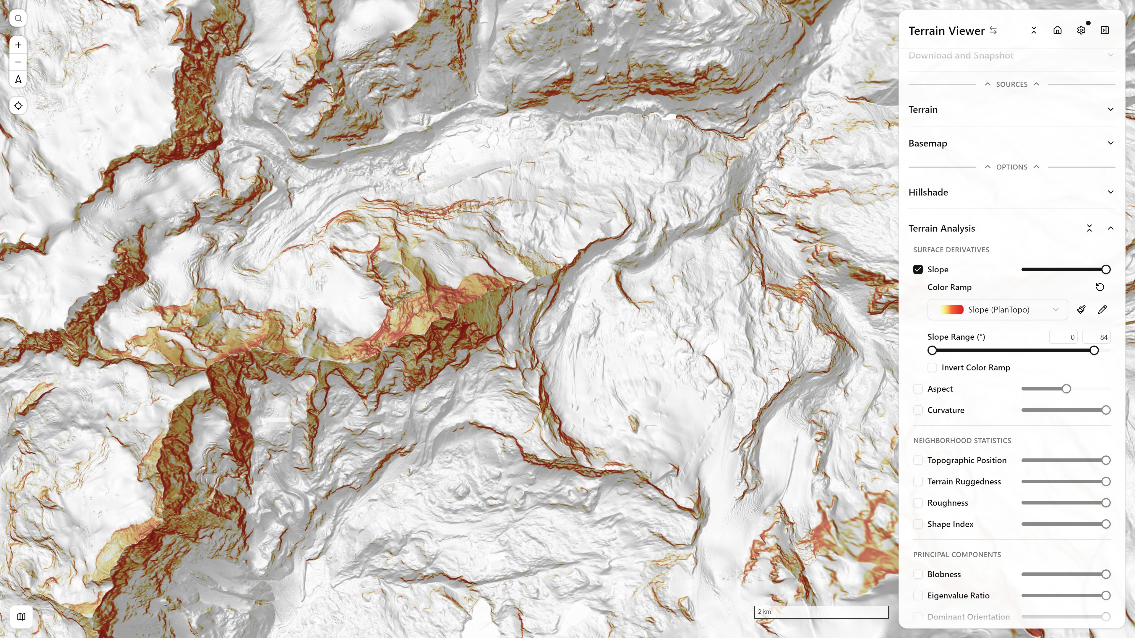
Terrain AnalysisCopy Anchor Link

See Terrain Analysis Rendering Pipeline and Equations & Formulas for how these are computed client-side from the raster-dem source.

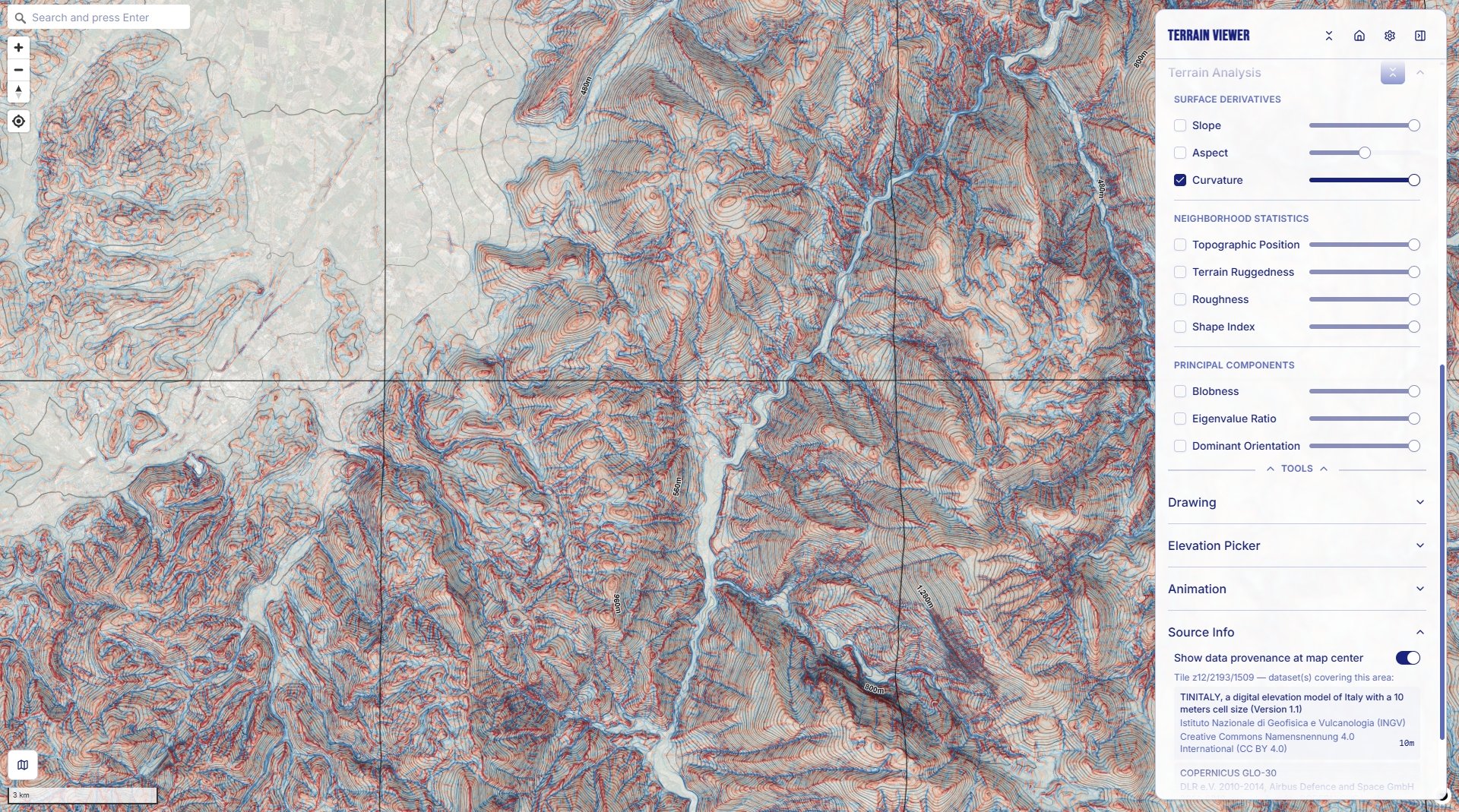
Terrain Analysis full submode list + Source Info provenance panel — Italian Alps

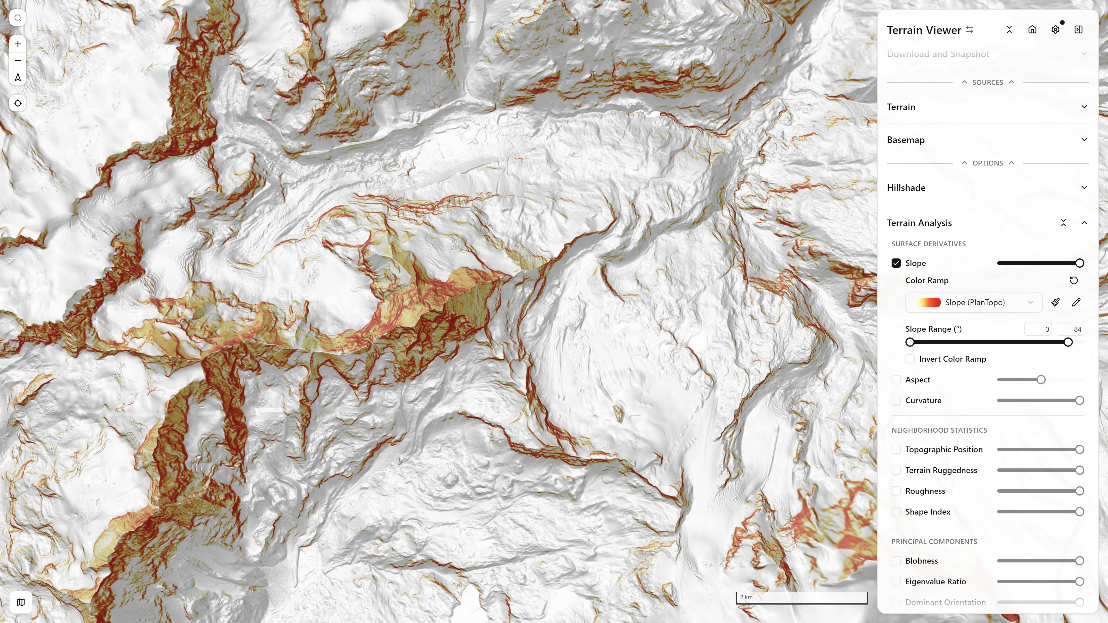
Terrain Analysis — Slope + Hillshade, with the Terrain Analysis controls panel open — Matterhorn massif — open in app ↗

• Slope — magnitude of the gradient
• Aspect — direction of the gradient
• Curvature — rate of slope change: Profile (flow acceleration), Plan/Divergence (flow convergence), Det Hessian (blob/saddle detector), or Combined (discrete Laplacian)
• TRI (Terrain Ruggedness Index) — mean elevation difference to neighbors
• TPI (Topographic Position Index) — elevation relative to the neighborhood mean
• Roughness — max − min elevation in a neighborhood
• Blobness — structure-tensor measure of gradient-direction variance; high at peaks/pits/saddles/knolls
• Shape Index, Eigen Ratio, Orientation — further curvature-tensor-derived shape descriptors

Relief VisualizationCopy Anchor Link

SVF/Openness/Local Dominance share the terrain-analysis pipeline above (just a ray-marched kernel instead of a 3×3 one); LRM's pyramid-ancestor mechanism is different enough to get its own page.

• LRM (Local Relief Model) — raw elevation minus a low-pass-filtered version, isolating small features from large-scale topography (the low-pass layer comes from a coarser pyramid tile, bilinearly upsampled)
• Sky-View Factor (SVF) — fraction of the visible sky hemisphere from each point (low in enclosed pits/canyons, high on open summits/ridges), from a ray-marched horizon angle in 8 directions (Zakšek, Oštir & Kokalj, 2011)
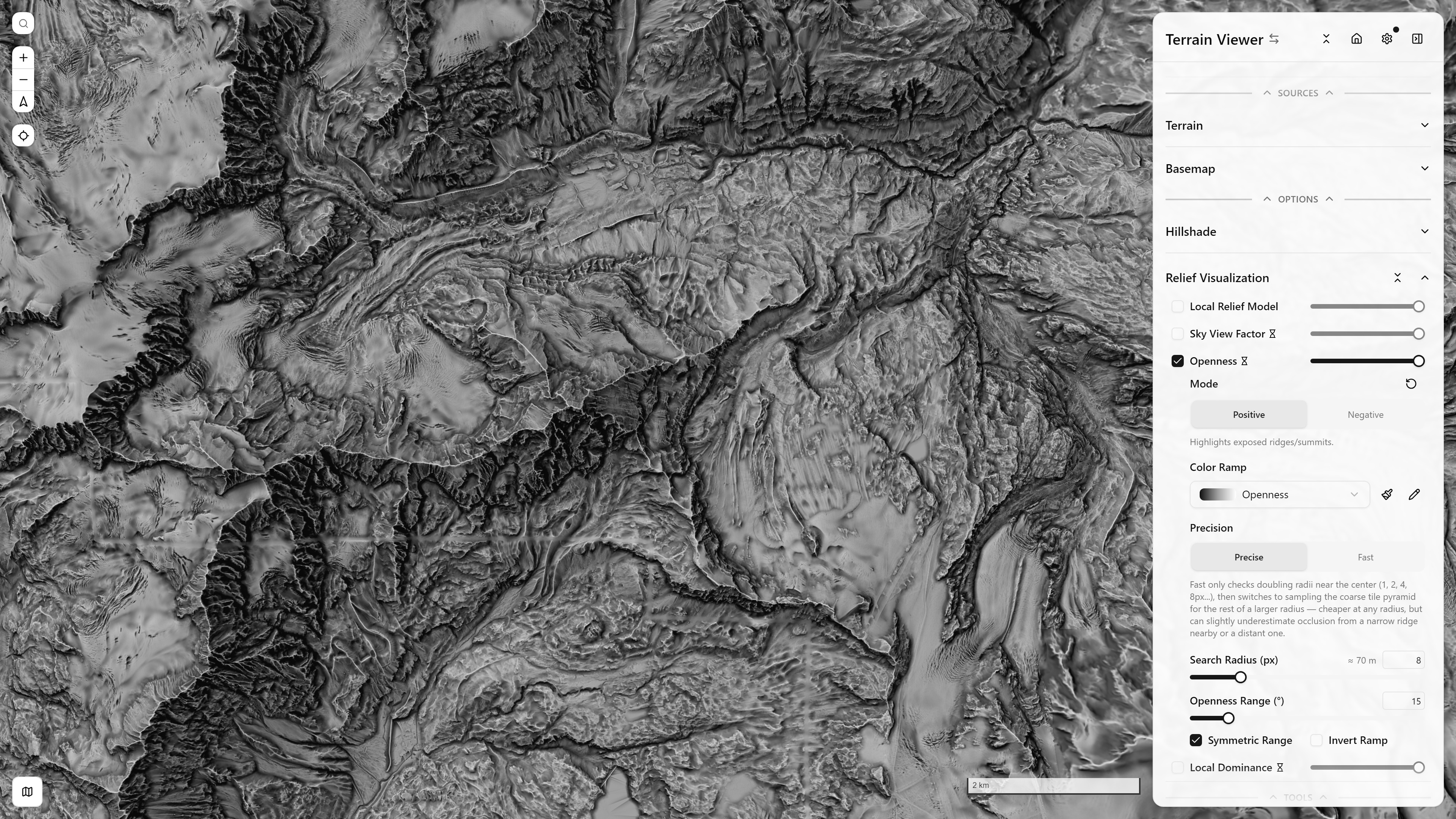
• Openness — mean angular distance from zenith to the horizon across the same 8 directions; Positive highlights ridges/summits, Negative highlights valleys/pits
• Local Dominance — local visibility-weighted elevation contrast

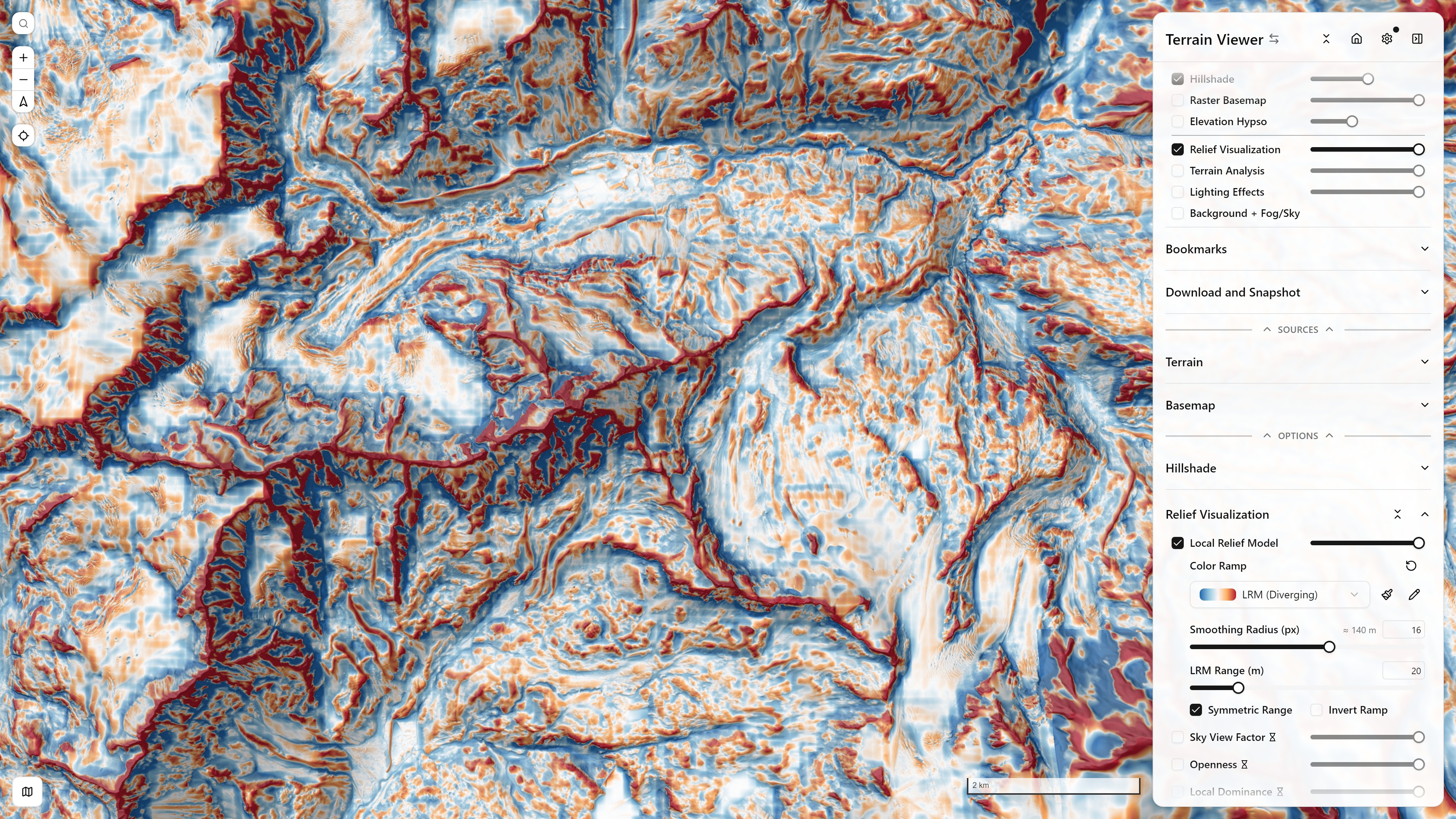
Relief Visualization — LRM + Hillshade, with the Relief Visualization controls panel open — Matterhorn massif — open in app ↗

Lighting EffectsCopy Anchor Link

See Lighting Effects for how these differ from the terrain-analysis pipeline above (real surface normals, GPU shading, a live-WebGL fast path), and Sun Position for the astronomy behind driving Phong's light from real solar position.

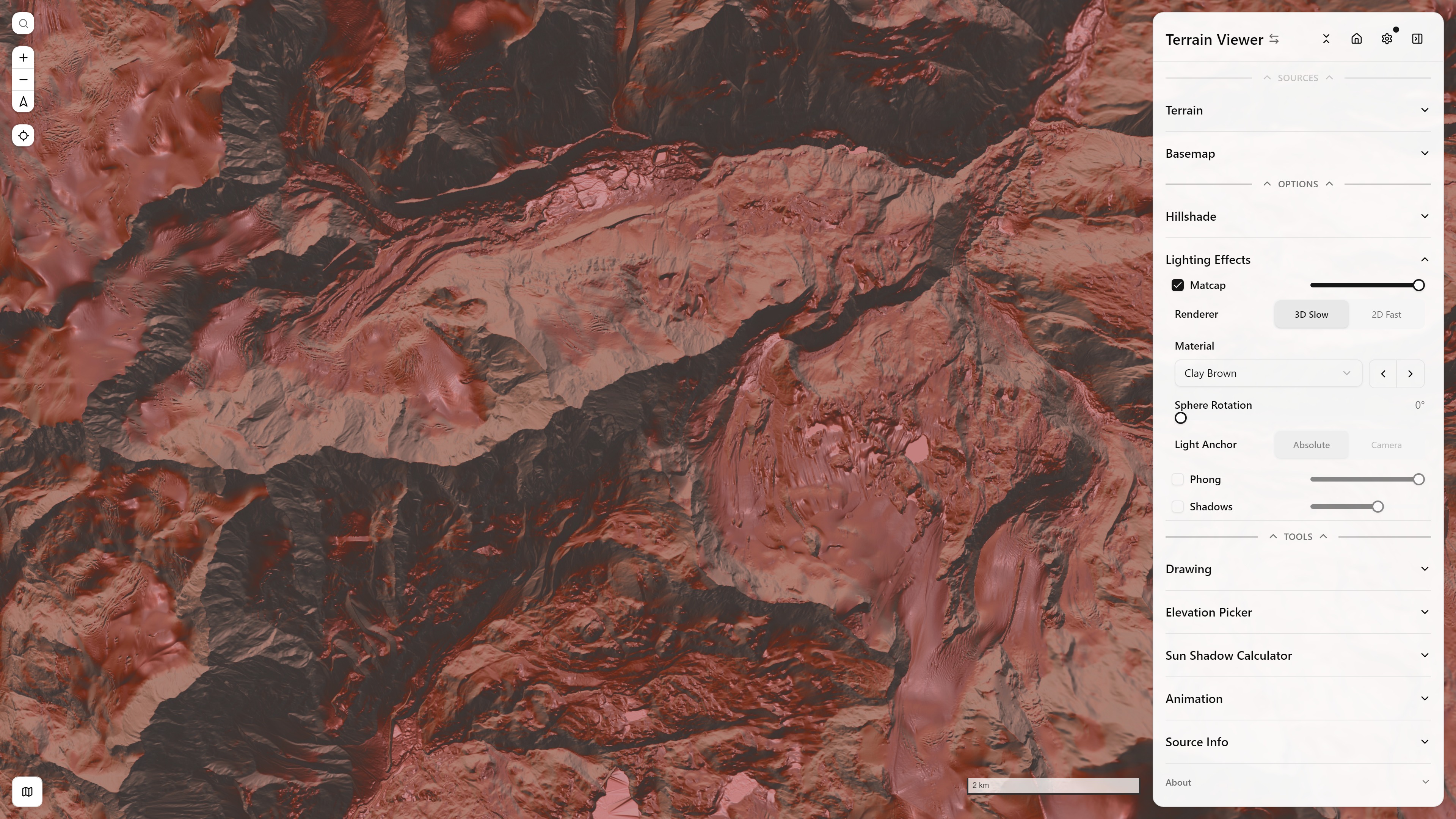
• Matcap — material-capture-style shading looked up by surface normal, independent of any real light direction; the Duotone Sphere material matches the Duotone NW/NE hillshade
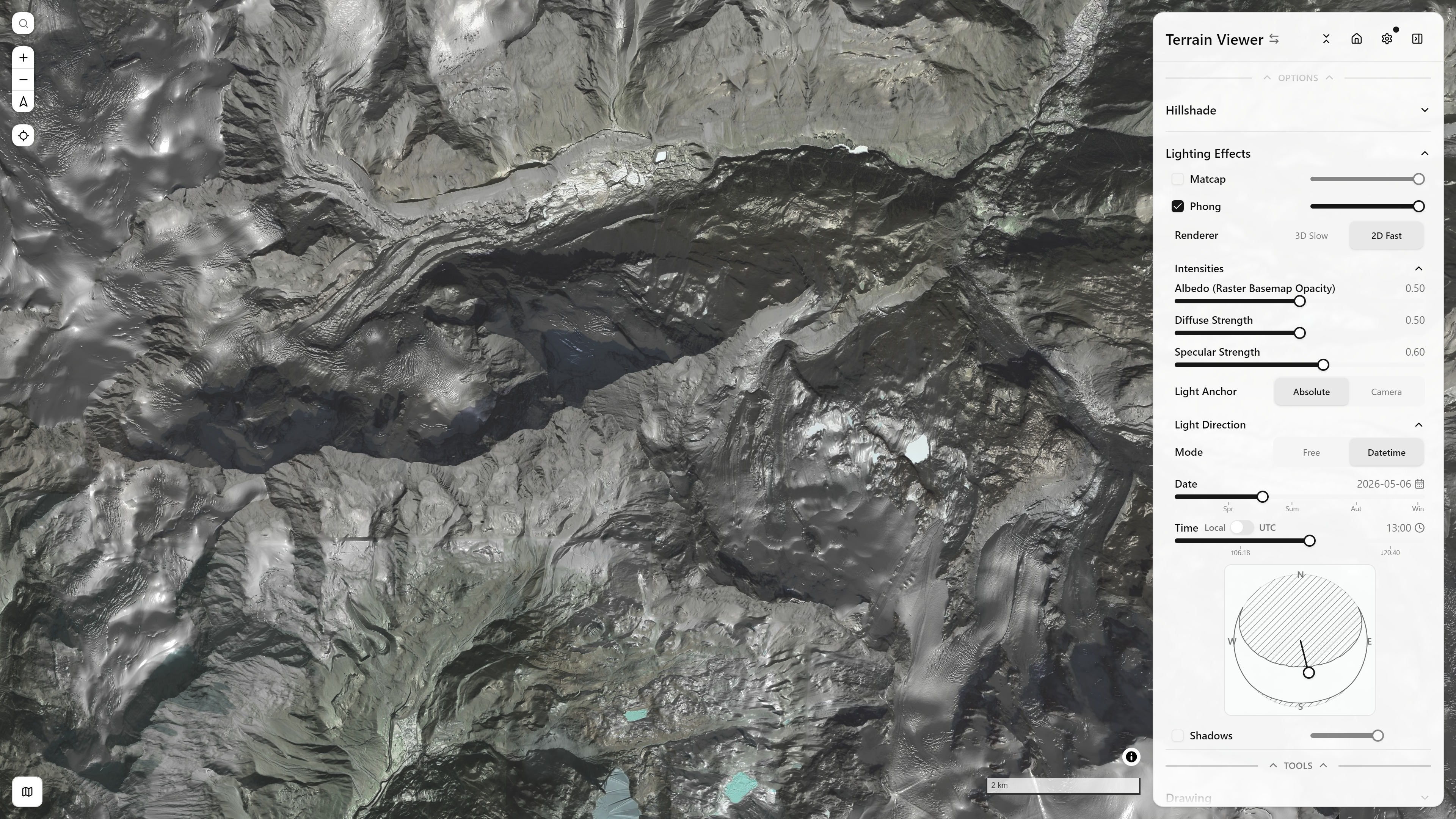
• Phong — ambient + diffuse + specular shading from a compass-fixed (or camera-relative) light, sharing the "hold L, drag" on-map light control. With the live renderer it takes up to three coloured lights: in Free mode, Light Direction shows Lights 1 / 2 / 3 and a colour swatch per light, and lights 2 and 3 are pills of their colour on the light pad (blue from the north-east and orange from the south-east by default). Fresnel Rim (under Intensities, with Rim Falloff) brightens the edges of slopes that turn away from the camera; it shows best on a tilted view. Details in Lighting Effects.
• Shadows, two kinds sharing one light (the same pad, or the datetime sun):
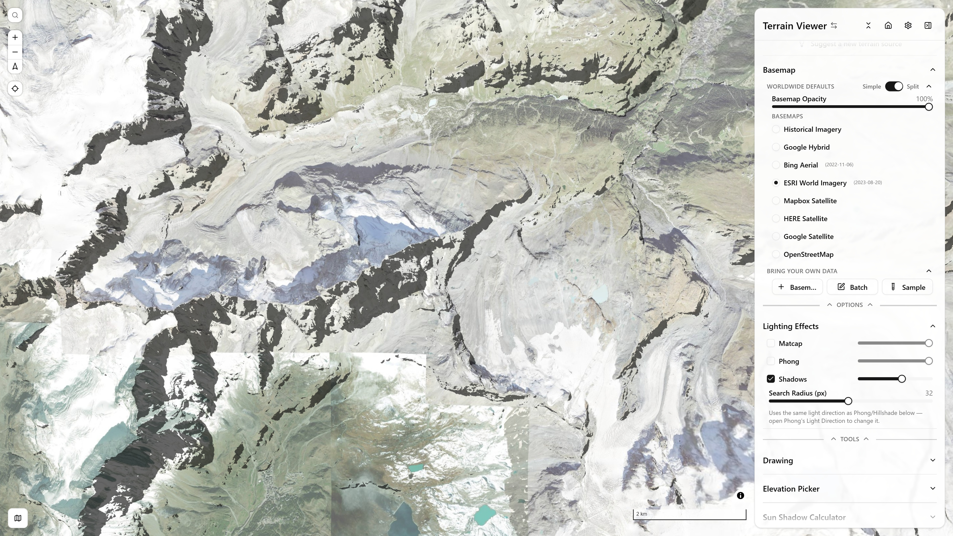
  • Terrain (hard shadows) — cast shadows from a single ray marched toward the sun's actual azimuth/altitude
  • Buildings (OSM) — shadows of OpenStreetMap buildings (heights from OpenFreeMap's building layer, OSM height or levels), the fast flat-ground way, on the GPU: each footprint is swept away from the sun by height / tan(altitude), the sweeps are drawn once into a mask (overlaps never darken twice, roofs stay lit), and the mask is composited over the map. The buildings are read once per settled view, from zoom 13; moving the light is a repaint, so the sun slider is live. Needs no OSM basemap on. Mercator only, and over 3D terrain the shadows stay on the flat plane the buildings' feet are drawn on; for shadows cast by the real shapes (a spire, a dome) falling on slopes, use the terrain Shadows above with a surface model (DSM) as the terrain source. Off by default (showBuildingShadows=true, buildingShadowOpacity).

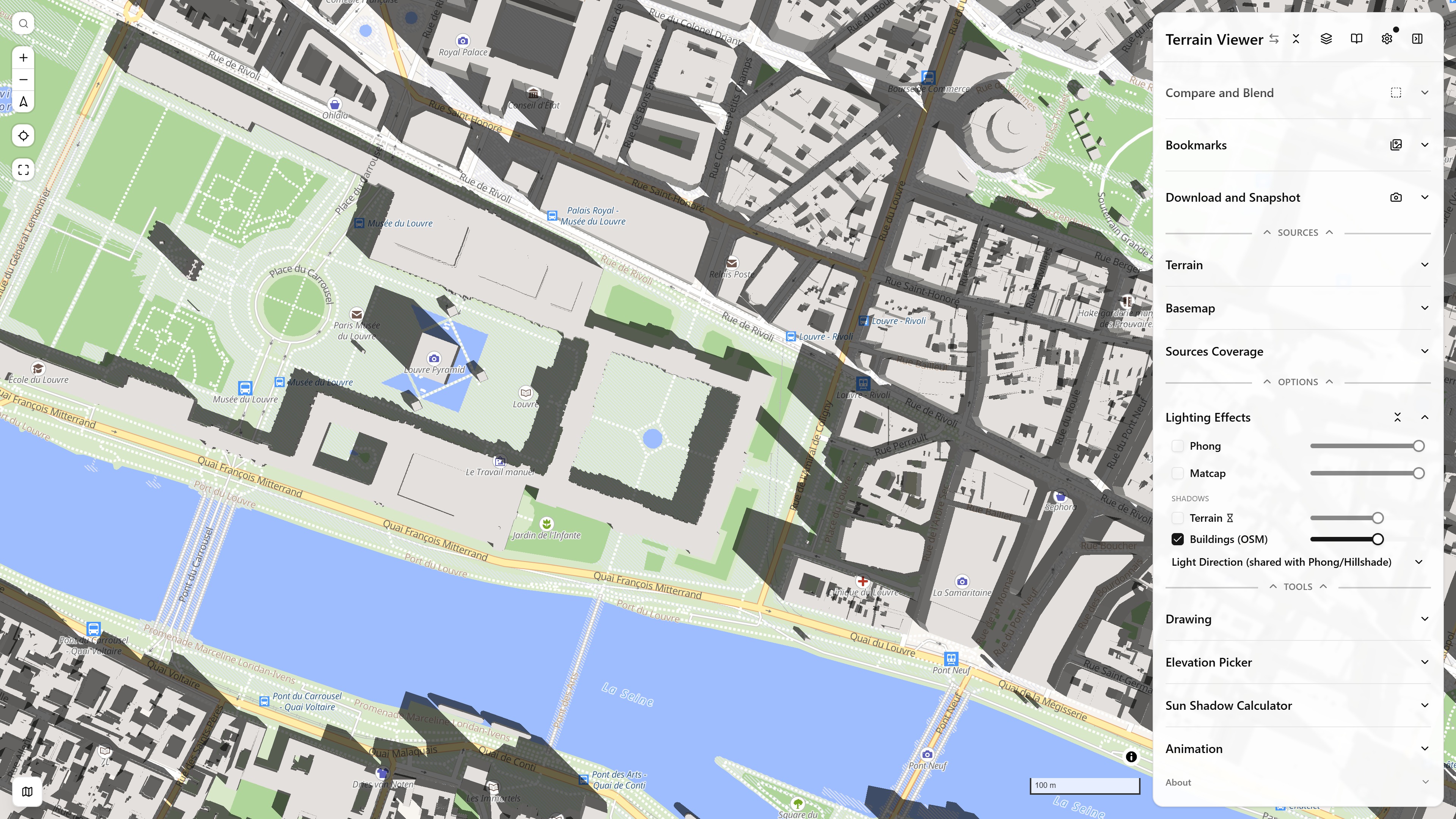
Lighting Effects, Shadows → Buildings (OSM), sun from the south-east at 20°, on the OpenStreetMap basemap, the Louvre, Paris · open in app ↗

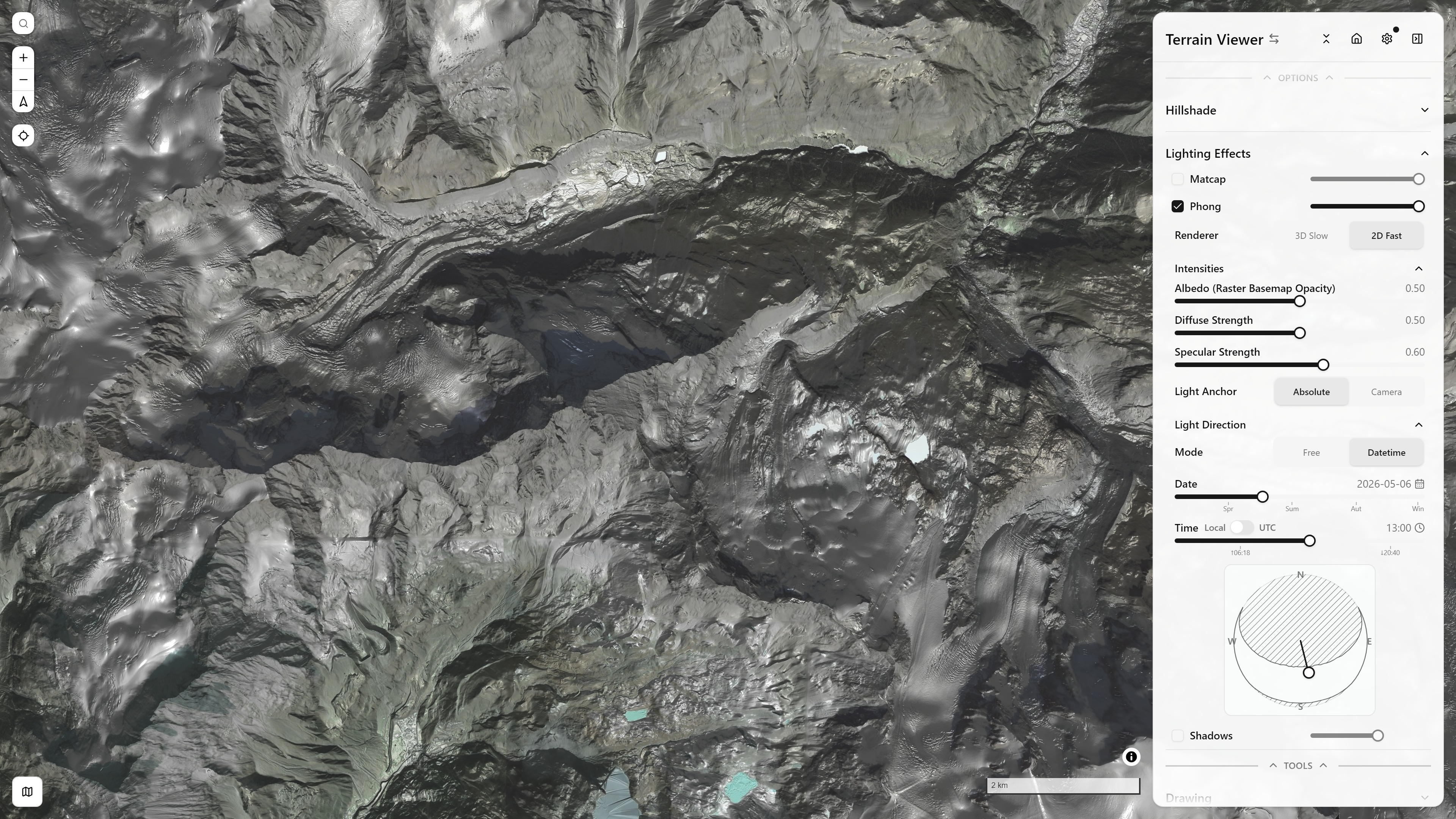
Lighting Effects — Phong + Hillshade + Raster Basemap, Datetime-driven light direction, with the Lighting Effects controls panel open — Matterhorn massif — open in app ↗

Tells (Mound Candidate) Detection — BetaCopy Anchor Link

Computes a Difference-of-Gaussians of the LRM as the primary bump signal, keeps only its local maxima (non-maximum suppression scaled to the configured tell size), then vetoes candidates failing any of three shape filters (Blobness, Plan Curvature, Det-Hessian). Opt in via Settings or ?tellsBeta=true.

Full ReferenceCopy Anchor Link

The same description shown in the app's own Settings → Visualization Modes:

Grouped as they are in the panel — Terrain Analysis (surface derivatives + neighborhood statistics), Relief Visualization (multi-scale relief / visibility) and Light (normal-based shading). Most are supported by — and inspired by — gdaldem and the RVT (Relief Visualization Toolbox) QGIS plugin (Kokalj & Hesse 2017 is its guide). Each mode links its original paper; more on Research References.

Terrain Analysis

Surface derivatives

• Slope: magnitude of the gradient, by Horn's 3×3 method as in gdaldem (Horn 1981)
• Aspect: direction of the gradient (Horn 1981)
• Curvature: rate of slope change — Profile, Plan, Mean/Combined, Gaussian (Det Hessian), or Casorati (Zevenbergen & Thorne 1987; definitions in Minár et al. 2020)
  • Profile (Flow Acceleration): rate of slope change along the steepest-descent direction, affects flow acceleration
  • Plan (Convergence/Divergence): rate of aspect change across contours, affects flow convergence/divergence — equivalent to the divergence of the normalized gradient field, div(∇z/|∇z|)
  • Mean/Combined: discrete Laplacian (∇²z) — mean curvature H = (κ₁+κ₂)/2, general surface bending that doesn't separate flow direction from contour direction
  • Gaussian Curvature (Det Hessian): determinant of the Hessian (fxx·fyy − fxy²) — Gaussian curvature K = κ₁·κ₂, a blob/saddle detector, positive at bowl/dome-shaped extrema and negative at saddle points
  • Casorati: κ = √((κ₁²+κ₂²)/2) — RMS of the two principal curvatures (Koch, 1993); always ≥ 0, measures how curved the surface is regardless of shape (dome, ridge, saddle, valley and bowl all read the same), zero only on flat ground

Neighborhood statistics

• TRI (Terrain Ruggedness Index): mean elevation difference to neighbors (Riley, DeGloria & Elliot 1999)
• TPI (Topographic Position Index): elevation relative to neighborhood mean (Weiss 2001; Guisan, Weiss & Weiss 1999; on archaeological landscapes, De Reu et al. 2013)
• Roughness: max−min elevation in a neighborhood
• Shape Index: SI = (2/π)·atan2(κ₁+κ₂, κ₁−κ₂) — Koenderink & van Doorn (1992); scale-free and bounded to [−1, 1] regardless of curvature magnitude: +1 dome/peak, +0.5 ridge, 0 saddle, −0.5 valley, −1 pit/bowl

Principal Components (PCA)

A local 2D PCA of the window's gradient vectors, via the Förstner/Harris structure tensor (box-averaged Ixx/Iyy/Ixy over a 5×5 window) — the same tensor behind all three modes below.

• Blobness: det(J)/trace(J) — large where the gradient direction varies in every direction (peaks, pits, saddles, knolls), near zero on a uniform slope or straight ridge/valley; conflates shape with steepness
• Eigenvalue Ratio: λmin/λmax of the structure tensor (0–100%) — shape only, independent of steepness: 0% is a coherent linear feature (slope/ridge/valley), 100% is an isotropic blob (peak/pit/saddle)
• Dominant Orientation: axis (0–180°) of the tensor's dominant eigenvector — which way a linear feature (ridge, valley, fault line) runs; most meaningful where Eigenvalue Ratio is low

Relief Visualization

• LRM (Local Relief Model): raw elevation minus a low-pass-filtered version, isolating small features from large-scale topography — the low-pass mean is bilinearly interpolated from a lower-resolution tile further up the pyramid tree. Conceptually close to HAG (Height Above Ground), but with the "ground" being that smoothed local trend surface rather than a classified bare-earth model (Hesse 2010).
• SVF (Sky-View Factor): the fraction of the sky hemisphere visible from a point (0–1), estimated from horizon angles sampled in many directions — darkens enclosed valleys and pits, brightens exposed ridges and summits, independent of any light direction (Zakšek, Oštir & Kokalj 2011)
• Openness (Positive / Negative): the mean zenith (positive) or nadir (negative) horizon angle over a search radius — positive openness emphasizes convex, exposed features (ridges, crests), negative openness emphasizes concave ones (channels, pits); a diffuse, illumination-free relief (Yokoyama et al. 2002; in archaeology, Doneus 2013)
• Local Dominance: how much a location visually towers over its surroundings — the mean angular drop to the terrain around it across a radius range, highlighting locally elevated features such as mounds, plateaus and terraces

Light

• Matcap (material capture): looks up a surface colour from a pre-lit sphere image using the surface normal as UV coordinates — a stylized, art-directable shading that doesn't depend on a directional light
• Phong: real ambient + diffuse + specular shading from a compass-fixed (or camera-relative) light direction — a physically-plausible 3D-relief render; the "Live" renderer is a per-fragment GPU shader draped on the terrain mesh, "Legacy" the raster-tile pipeline (still the globe-capable one) — see the Lighting Effects panel (Phong 1975)
• Shadows: hard cast shadows — darkens a pixel wherever nearby terrain rises above the sun's own angle in the sky, blocking direct light (a single-ray horizon-angle march toward the sun's azimuth); shares Phong/Hillshade's light direction, no separate control of its own beyond opacity and search radius

Neighborhood usually refers to a 3×3 kernel centered on the pixel.

Terrain Encoding Functions

TerrainRGB: height = -10000 + ((R * 256 * 256 + G * 256 + B) * 0.1)

Terrarium: height = (R * 256 + G + B / 256) - 32768